Build confidence with Spark
Apache Spark is a unified analytics engine for big data processing with a myriad of built-in modules for Machine Learning, Streaming, SQL, and Graph Processing. Learn about the best practices when creating Spark integration projects.
What is Spark? Apache Spark is a data processing framework that can quickly perform processing tasks on very large data sets, and can also distribute data processing tasks across multiple computers, either on its own or in tandem with other distributed computing tools
Apache Spark™ is a unified analytics engine for large-scale data processing at high speed and run workloads 100x faster. Apache Spark achieves high performance for both batch and streaming data, using a state-of-the-art DAG scheduler, a query optimizer, and a physical execution engine.
-
We can write spark applications quickly in Java, Scala, Python, R, and SQL. Spark offers over 80 high-level operators that make it easy to build parallel apps. And you can use it interactively from the Scala, Python, R, and SQL shells.
-
With Spark Read JSON files with automatic schema inference and Combine SQL, streaming, and do complex analytics. Spark powers a stack of libraries including SQL and DataFrames, MLlib for machine learning, GraphX, and Spark Streaming. You can combine these libraries seamlessly in the same application.
-
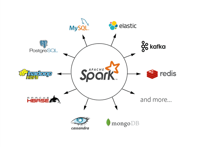
Spark runs on Hadoop, Apache Mesos, Kubernetes, standalone, or in the cloud. It can access diverse data sources.
The architecture of Apache Spark
-
Spark Driver (Master Process) The Spark Driver converts the programs into tasks and schedule the tasks for Executors. The Task Scheduler is the part of Driver and helps to distribute tasks to Executors.
-
Spark Cluster Manager A cluster manager is the core in Spark that allows to launch executors and sometimes drivers can be launched by it also. Spark Scheduler schedules the actions and jobs in Spark Application in FIFO way on cluster manager itself. You should also read about Apache Airflow.
-
Executors (Slave Processes) Executors are the individual entities on which individual task of Job runs. Executors will always run till the lifecycle of a spark Application once they are launched. Failed executors don’t stop the execution of spark job.
-
RDD (Resilient Distributed Datasets) An RDD is a distributed collection of immutable datasets on distributed nodes of the cluster. An RDD is partitioned into one or many partitions. RDD is the core of spark as their distribution among various nodes of the cluster that leverages data locality. To achieve parallelism inside the application, Partitions are the units for it. Repartition or coalesce transformations can help to maintain the number of partitions. Data access is optimized utilizing RDD shuffling. As Spark is close to data, it sends data across various nodes through it and creates required partitions as needed.
-
DAG (Directed Acyclic Graph) Spark tends to generate an operator graph when we enter our code to Spark console. When an action is triggered to Spark RDD, Spark submits that graph to the DAGScheduler. It then divides those operator graphs to stages of the task inside DAGScheduler. Every step may contain jobs based on several partitions of the incoming data. The DAGScheduler pipelines those individual operator graphs together. For Instance, Map operator graphs schedule for a single-stage and these stages pass on to the. Task Scheduler in cluster manager for their execution. This is the task of Work or Executors to execute these tasks on the slave.
-
Distributed processing using partitions efficiently Increasing the number of Executors on clusters also increases parallelism in processing Spark Job. But for this, one must have adequate information about how that data would be distributed among those executors via partitioning. RDD is helpful for this case with negligible traffic for data shuffling across these executors. One can customize the partitioning for pair RDD (RDD with key-value Pairs). Spark assures that set of keys will always appear together in the same node because there is no explicit control in this case.
Spark Program Execution Stages
A Spark job is divided into stages, defined by points where shuffles occur.
- For each stage, the driver creates tasks and sends them to the executors.
- The executors write their intermediate results to local disk. Shuffling is performed by special shuffle-map tasks.
- The last stage returns its results to the driver, using special results tasks.
When to use RDDs?
- Low-level API & control of dataset
- Dealing with unstrucrured data (media streams or texts)
- Manipulate data with lambda functions than DSL
- Don’t care schema or structure of data
- Sacrifice optimization, performance & inefficiecies
When to use Datasets/DataFrames
Starting in Spark 2.0, Dataset takes on two distinct APIs characteristics: a strongly-typed API and an untyped API, as shown in the table below. Conceptually, consider DataFrame as an alias for a collection of generic objects Dataset[Row], where a Row is a generic untyped JVM object. Dataset, by contrast, is a collection of strongly-typed JVM objects, dictated by a case class you define in Scala or a class in Java.
// convert RDD -> DF with column names
val df = parsedRDD.toDF("project", "page", "numRequests")
//filter, groupBy, sum, and then agg()  df.filter($"project" === "en").
groupBy($"page").  agg(sum($"numRequests").as("count")).
limit(100).  show(100)

//output
project  page  numRequests
en       23         45
en       24         200
- If you want rich semantics, high-level abstractions, and domain specific APIs, use DataFrame or Dataset.
- If your processing demands high-level expressions, filters, maps, aggregation, averages, sum, SQL queries, columnar access and use of lambda functions on semi-structured data, use DataFrame or Dataset.
- If you want higher degree of type-safety at compile time, want typed JVM objects, take advantage of Catalyst optimization, and benefit from Tungsten’s efficient code generation, use Dataset.
- If you want unification and simplification of APIs across Spark Libraries, use DataFrame or Dataset.
- If you are a R user, use DataFrames.
- If you are a Python user, use DataFrames and resort back to RDDs if you need more control.
DataFrame
data.groupBy("dept").avg("age")

SQL
select	dept,	avg(age)	from	data	group	by	1

RDD
data.map	{ case	(dept,	age)	=>  dept	-> (age,	1) }
.reduceByKey	{ case	((a1,	c1),	(a2,	c2)) =>	(a1 + a2, c1 + c2)}
.map	{ case	(dept,	(age,	c)) =>  dept	-> age	/ c }
DataFrame Optimization
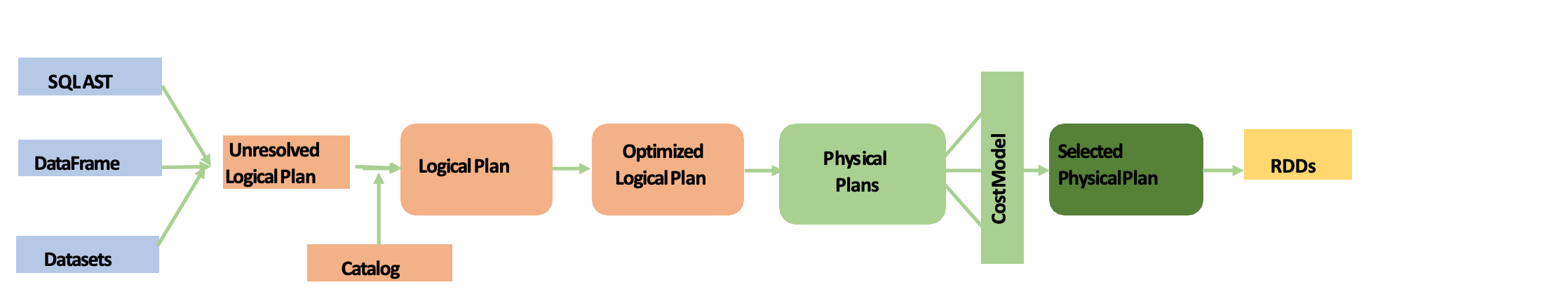
Catalyst Optimizer
-
Analysis: analyzing a logical plan to resolve references
-
Logical Optimization: logical plan optimization
-
Physical Planning: Physical planning
-
Code Generation: Compile parts of the query to Java bytecode
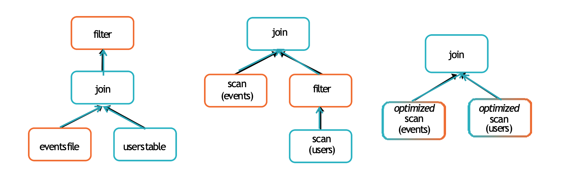
users.join(events, users("id") === events("uid")) . filter(events("date") > "2015-01-01")
Tungsten - Optimization Project
-
Project Tungsten's goal was to improve Spark execution by optimising Spark jobs for CPU and memory efficiency (as opposed to network and disk I/O which are considered fast enough). It offers benefits such as Off-Heap Memory Management using binary in-memory data representation aka Tungsten row format and managing memory explicitly, Cache Locality which is about cache-aware computations with cache-aware layout for high cache hit rates and Whole-Stage Code Generation (aka CodeGen).
-
Sharing data from one worker to another can be a costly operation. Spark has optimized this operation by using a format called Tungsten. Tungsten prevents the need for expensive serialization and de-serialization of objects in order to get data from one JVM to another. The data that is "shuffled" is in a format known as UnsafeRow, or more commonly, the Tungsten Binary Format. UnsafeRow is the in-memory storage format for Spark SQL, DataFrames & Datasets. The benefit of using Spark 2.x's custom encoders is that you get almost the same compactness as Java serialization, but significantly faster encoding/decoding speeds. Spark can operate directly out of Tungsten, without first deserializing Tungsten data into JVM objects.
Spark Transformations
Spark Transformation is a function that produces new RDD from the existing RDDs. It takes RDD as input and produces one or more RDD as output. Each time it creates new RDD when we apply any transformation. Thus, the so input RDDs, cannot be changed since RDD are immutable in nature.
Not all transformations are born equal. Some are more expensive than others and if you shuffling data all around you cluster network, then you performance you surely take the hit! In order to understand why some transformations can have this impact into the execution time, we need to understand the basic difference between narrow and long dependencies in Apache Spark.
Applying transformation built an RDD lineage, with the entire parent RDDs of the final RDD(s). RDD lineage, also known as RDD operator graph or RDD dependency graph. It is a logical execution plan i.e., it is Directed Acyclic Graph (DAG) of the entire parent RDDs of RDD.
Transformations are lazy in nature i.e., they get execute when we call an action. They are not executed immediately. Two most basic type of transformations is a map(), filter(). After the transformation, the resultant RDD is always different from its parent RDD. It can be smaller (e.g. filter, count, distinct, sample), bigger (e.g. flatMap(), union(), Cartesian()) or the same size (e.g. map).
-
There are two types of transformations:
-
Narrow transformation
In Narrow transformation, all the elements that are required to compute the records in single partition live in the single partition of parent RDD. A limited subset of partition is used to calculate the result. Narrow transformations are the result of map(), filter().
-
Wide transformation
In wide transformation, all the elements that are required to compute the records in the single partition may live in many partitions of parent RDD. The partition may live in many partitions of parent RDD. Wide transformations are the result of groupbyKey() and reducebyKey().
A shuffle can occur when the resulting RDD depends on other elements from the same RDD or another RDD. In fact, RDD dependencies encode when data must move across network. Thus they tell us when data is going to be shuffled.
-
-
Transformations cause shuffles, and can have 2 kinds of dependencies:
-
Narrow dependencies: Each partition of the parent RDD is used by at most one partition of the child RDD.
[parent RDD partition] ---> [child RDD partition]Fast! No shuffle necessary. Optimizations like pipelining is an option. Thus transformations which have narrow dependencies are fast.
-
-
Wide dependencies: Each partition of the parent RDD may be used by multiple child partitions
                    ---> [child RDD partition 1]
[parent RDD partition] ---> [child RDD partition 2]
                    ---> [child RDD partition 3]
Slow! Shuffle necessary for all or some data over the network. Thus transformations which have narrow dependencies are slow. Thus operations like join can sometimes be narrow and sometimes be wide.
Transformations with Narrow dependencies:
map()
mapValues()
flatMap()
filter()
mapPartitions()
mapPartitionsWithIndex()
Transformations with Wide dependencies: (might cause a shuffle)
cogroup()
groupWith()
join()
leftOuterJoin()
rightOuterJoin()
groupByKey()
reduceByKey()
combineByKey()
distinct()
intersection()
repartition()
coalesce()
Spark splits data into partitions and computation is done in parallel for each partition. It is very important to understand how data is partitioned and when you need to manually modify the partitioning to run spark applications efficiently.
Partitioning in Apache Spark
One important way to increase parallelism of spark processing is to increase the number of executors on the cluster. However, knowing how the data should be distributed, so that the cluster can process data efficiently is extremely important. The secret to achieve this is partitioning in Spark. Apache Spark manages data through RDDs using partitions which help parallelize distributed data processing with negligible network traffic for sending data between executors. By default, Apache Spark reads data into an RDD from the nodes that are close to it.
val rdd= sc.textFile (“file.txt”, 5)

Scala> rdd.partitions.size
Output = 5
What is Coalesce?
The coalesce method reduces the number of partitions in a DataFrame. Coalesce avoids full shuffle, instead of creating new partitions, it shuffles the data using Hash Partitioner (Default), and adjusts into existing partitions, this means it can only decrease the number of partitions.
Coalesce use case: we pass in all N partitions into the RDD and perform some action, the partition which processes the file part-00000 will finish first followed by others but the executor with part-00005 will be still running meanwhile 1st executor will be idle. Hence, the load is not balanced on executors equally.
What is Repartitioning?
The repartition method can be used to either increase or decrease the number of partitions in a DataFrame. Repartition is a full Shuffle operation, whole data is taken out from existing partitions and equally distributed into newly formed partitions.
Repartition use case: All the executors finish the job at the same time, and the resources are consumed equally because all input partitions have the same size.
What is Checkpointing?
Checkpointing is the act of saving an RDD to disk so that future references to this RDD point to those intermediate partitions on disk rather than recomputing the RDD from its original source. This is similar to caching except that it’s not stored in memory, only disk. use Checkpointing, if the results of a set of transformations (history) can be reused for a long time. If the answer is no, use caching.
An example where checkpointing is beneficial when crunching a RDD or DataFrame of taxes for a previous year. The data is unlikely to change once calculated so it would be much better to checkpoint and save it forever for reuse.
What is Caching?
Spark Cache and Persist are optimization techniques in DataFrame / Dataset for iterative and interactive Spark applications to improve the performance of Jobs. Caching is extremely effective and more useful than checkpointing, as it’s typically much faster when used properly, when you have a lot of available memory. RDDs and DataFrames can be massive in size, like giga or terabyte size. Essentially, caching will maintain the result of applying a set of transformations to an RDD or DataFrame so that those transformations do not have to be recomputed again when an additional transformation is applied or fault occurs within a RDD or DataFrame.
An example where caching would be appropriate would be like calculating the power usage of homes for a day: any transformations that need to be made to a RDD or DataFrame to determine the power usage for homes for a day are most likely going to be unique day and would never be used again for any following day’s calculations.
The sorts of dependency objects that this method may return include:
-
Narrow dependency objects
- OneToOneDependency
- PruneDependency
- RangeDependency
-
Wide dependency objects
- ShuffleDependency
val wordsRDD = sc.parallelize(largeList)

/* dependencies */

val pairs = wordsRdd.map(c=>(c,1))
                    .groupByKey
                    .dependencies          // <-------------
// pairs: Seq[org.apache.spark.Dependency[_]] = List(org.apache.spark.ShuffleDependency@4294a23d)

/* toDebugString */

val pairs = wordsRdd.map(c=>(c,1))
                    .groupByKey
                    .toDebugString         // <-------------
// pairs: String =
// (8) ShuffledRDD[219] at groupByKey at <console>:38 []
//  +-(8) MapPartitionsRDD[218] at map at <console>:37 []
//     | ParallelCollectionRDD[217] at parallelize at <console>:36 []
Shuffling in Spark
A shuffle occurs when data is rearranged between partitions. This is required when a transformation requires information from other partitions, such as summing all the values in a column. Spark will gather the required data from each partition and combine it into a new partition, likely on a different executor. Shuffling is a mechanism Spark uses to redistribute the data across different executors and even across machines. Spark shuffling triggers when we perform certain transformation operations like gropByKey(), reducebyKey(), join() on RDD and DataFrame.
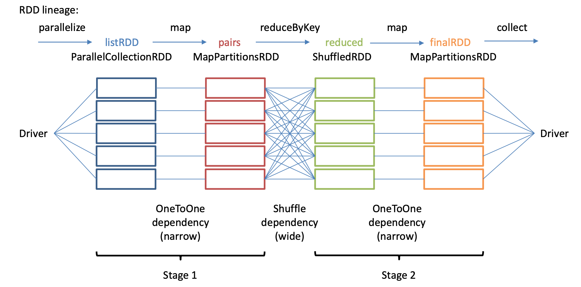
val myList = List.fill(500) (scala.util.Random.nextInt(10) )
val listRDD = sc.parallelize(myList, 5) // creates 5 partitions of the list
val pairs = listRDD.map(x => (x, x*x) )
val reduced = pairs.reduceByKey( (v1, v2) => (v1+v2) )
val finalRDD = reduced.mapPartitions( iter => iter.map({case(k, v) => “K=“+k+”, V=“+v}) ).collect()
Deeper Dive into Shuffling
-
Spark Shuffle is central for opeartions when a reorganization of data is required. It is an expensive operation since it involves the following:
- Disk I/O
- Involves data serialization and deserialization
- Network I/O
- When creating an RDD, Spark doesn’t necessarily store the data for all keys in a partition since at the time of creation there is no way we can set the key for data set.
Steps to shuffle data
- Convert the data to the UnsafeRow, commonly referred to as Tungsten Binary Format.
- Write that data to disk on the local node - at this point the slot is free for the next task.
- Driver decides which executor gets which piece of data.
- Spark first runs map tasks on all partitions which groups all values for a single key.
- The results of the map tasks are kept in memory.
- When results do not fit in memory, Spark stores the data into a disk.
- Spark shuffles the mapped data across partitions, some times it also stores the shuffled data into a disk for reuse when it needs to recalculate.
- Then the executor pulls the data it needs from the other executor's shuffle files.
- Run the garbage collection
- Finally runs reduce tasks on each partition based on key.
Spark RDD triggers shuffle and repartition for several operations like repartition(), coalesce(), groupByKey(), reduceByKey(), cogroup() and join() but not countByKey(). Both getNumPartitions from the above examples return the same number of partitions. Though reduceByKey() triggers shuffle but results in the same number of partitions as parent RDD.
val spark:SparkSession = SparkSession.builder()
    .master("local[5]")
    .appName("SparkByExamples.com")
    .getOrCreate()

  val sc = spark.sparkContext

  val rdd:RDD[String] = sc.textFile("src/main/resources/test.txt")

  println(rdd.getNumPartitions)
  val rdd2 = rdd.flatMap(f=>f.split(" "))
  .map(m=>(m,1))

  //ReduceBy transformation
  val rdd5 = rdd2.reduceByKey(_ + _)

  println(rdd5.getNumPartitions)
Unlike RDD, Spark SQL DataFrame API increases the partitions when the operation performs shuffling. This outputs the partition count as 200. DataFrame increases the partition number to 200 automatically when Spark operation performs data shuffling. The default shuffle partition number comes from Spark SQL configuration spark.sql.shuffle.partitions which is by default set to 200. You can change this default shuffle partition value using conf method of the SparkSession object.
spark.conf.set("spark.sql.shuffle.partitions",100)
println(df.groupBy("_c0").count().rdd.partitions.length)
Shuffle partition size
Based on your dataset size, number of cores, and memory, Spark shuffling can benefit or harm your jobs. When you dealing with less amount of data, you should typically reduce the shuffle partitions otherwise you will end up with many partitioned files with a fewer number of records in each partition. which results in running many tasks with lesser data to process.
On other hand, when you have too much of data and having less number of partitions results in fewer longer running tasks and some times you may also get out of memory error.
Getting a right size of the shuffle partition is always tricky and takes many runs with different value to achieve the optimized number. This is one of the key property to look for when you have performance issues on Spark jobs.
val spark:SparkSession = SparkSession.builder()
    .master("local[1]")
    .appName("SparkByExamples.com")
    .getOrCreate()

  import spark.implicits._

  val simpleData = Seq(("James","Sales","NY",90000,34,10000),
    ("Michael","Sales","NY",86000,56,20000),
    ("Robert","Sales","CA",81000,30,23000),
    ("Maria","Finance","CA",90000,24,23000),
    ("Raman","Finance","CA",99000,40,24000),
    ("Scott","Finance","NY",83000,36,19000),
    ("Jen","Finance","NY",79000,53,15000),
    ("Jeff","Marketing","CA",80000,25,18000),
    ("Kumar","Marketing","NY",91000,50,21000)
  )
  val df = simpleData.toDF("employee_name","department","state","salary","age","bonus")

  val df2 = df.groupBy("state").count()

 println(df2.rdd.getNumPartitions)
Shuffle - writing side
The first important part on the writing side is the shuffle stage detection in DAGScheduler. To recall, this class is involved in creating the initial Directed Acyclic Graph for the submitted Apache Spark application. It's later divided into jobs, stages and tasks, and all those parts are sent to the resource manager for the physical execution.
DAGScheduler has a method called getShuffleDependencies(RDD) where it will retrieve all parent shuffle dependencies for given RDD. How are these dependencies found? In the physical plan, the shuffle nodes are represented by ShuffleExchangeExec and inside it, you can find a field called shuffleDependency. It holds a ShuffleDependency class involved in the shuffle stages detection at the DAGScheduler level.
The ShuffleDependency instance is created in the ShuffleExchangeExec as ShuffleDependency[Int, InternalRow, InternalRow] where the Int is the partition number, the first InternalRow is the corresponding row and the last one the combined rows after the shuffle. The partition here is the after-shuffle partition number, so the reader's partition that will need the row. And it's computed from a partitioner that can be one of RoundRobinPartitioning, HashPartitioning, RangePartitioning or SinglePartition. For the group by key operation, the partitioner will be the hash-based one and the partition will be computed from the modulo-based hash algorithm
Shuffle - reading side
As you can see, every "data" file, so the one storing the rows to fetch by the reducer at the reading stage, has a corresponding "index" file. Here, the BypassMergeSortShuffleWriter generated the output, but as announced, you will learn in another post whether this is different for other writers.
On the reader's side, the DAGScheduler executes the ShuffledRDD holding the ShuffleDependency introduced in the previous section. When it happens, the compute(split: Partition, context: TaskContext) method will return all records that should be returned for the Partition from the signature. And that's where the shuffle is, so the data transfers across the network (so far it remains local!). The compute method will create a ShuffleReader instance that will be responsible, through its read() method, to return an iterator storing all rows that are set for the specific reducer's.
Five best practices of Apache Spark Shuffling to build predictable, reliable and efficient Spark Applications
-
Data Re-distribution
-
Data Re-distribution is the primary goal of shuffling operation in Spark. Therefore, Shuffling in a Spark program is executed whenever there is a need to re-distribute an existing distributed data collection represented either by an RDD, Dataframe, or Dataset.
-
Increase or Decrease the number of data partitions: Since a data partition represents the quantum of data to be processed together by a single Spark Task, there could be situations:
(a) Where existing number of data partitions are not sufficient enough in order to maximize the usage of available resources.
(b) Where existing number of data partitions are too heavy to be computed reliably without memory overruns.
(c) Where existing number of data partitions are too high in number such that task scheduling overhead becomes the bottleneck in the overall processing time.
-
In all of the above situations, redistribution of data is required to either increase or decrease the number of underlying data partitions. The same is achieved by executing shuffling on the existing distributed data collection via commonly available ‘repartition’ API among RDDs, Datasets, and Dataframes.
-
Perform Aggregation/Join on a data collection(s): In order to perform aggregation/join operation on data collection(s), all data records belonging to aggregation, or a join key should reside in a single data partition. Therefore, if the existing partitioning scheme of the input data collection(s) does not satisfy the condition, then re-distribution in accordance with aggregation/join key becomes mandatory, and therefore shuffling would be executed on the input data collection to achieve the desired re-distribution.
-
-
-
Partitioner and Number of Shuffle Partitions Partitioner and number of shuffle partitions are other two important aspects of Shuffling. The number of shuffle partitions specifies the number of output partitions after the shuffle is executed on a data collection, whereas Partitioner decides the target shuffle/output partition number (out of the total number of specified shuffle partitions) for each of the data records. Spark APIs (pertaining to RDD, Dataset or Dataframe) which triggers shuffling provides either of implicit or explicit provisioning of Partitioner and/or number of shuffle partitions.
-
Shuffle Block A shuffle block uniquely identifies a block of data which belongs to a single shuffled partition and is produced from executing shuffle write operation (by ShuffleMap task) on a single input partition during a shuffle write stage in a Spark application. The unique identifier (corresponding to a shuffle block) is represented as a tuple of ShuffleId, MapId and ReduceId. Here, ShuffleId uniquely identifies each shuffle write/read stage in a Spark application, MapId uniquely identifies each of the input partition (of the data collection to be shuffled) and ReduceId uniquely identifies each of the shuffled partition.
-
Shuffle Read/Write A shuffle operation introduces a pair of stage in a Spark application. Shuffle write happens in one of the stage while Shuffle read happens in subsequent stage. Further, Shuffle write operation is executed independently for each of the input partition which needs to be shuffled, and similarly, Shuffle read operation is executed independently for each of the shuffled partition.
Shuffle read operation is executed using ‘BlockStoreShuffleReader’ which first queries for all the relevant shuffle blocks and their locations. This is then followed by pulling/fetching of those blocks from respective locations using block manager module. Finally, a sorted iterator on shuffled data records derived from fetched shuffled blocks is returned for further use.
Shuffle write operation (from Spark 1.6 and onward) is executed mostly using either ‘SortShuffleWriter’ or ‘UnsafeShuffleWriter’. The former is used for RDDs where data records are stored as JAVA objects, while the later one is used in Dataframes/Datasets where data records are stored in tungusten format. Both shuffle writers produces a index file and a data file corresponding to each of the input partition to be shuffled. Index file contains locations inside data file for each of the shuffled partition while data file contains actual shuffled data records ordered by shuffled partitions.
-
Shuffle Spill During shuffle write operation, before writing to a final index and data file, a buffer is used to store the data records (while iterating over the input partition) in order to sort the records on the basis of targeted shuffled partitions. However, if the memory limits of the aforesaid buffer is breached, the contents are first sorted and then spilled to disk in a temporary shuffle file. This process is called as shuffle spilling. Disk spilling of shuffle data although provides safeguard against memory overruns, but at the same time, introduces considerable latency in the overall data processing pipeline of a Spark Job. This latency is due to the fact that spills introduces additions disk read/write cycles along with ser/deser cycles (in case where data records are JAVA objects) and optional comp/decomp cycles. Amount of shuffle spill (in bytes) is available as a metric against each shuffle read or write stage. This spilling information could help a lot in tuning a Spark Job.
Spark's Python DataFrame API example:
df = spark.read.json("logs.json") df.where("age > 21") .select("name.first").show()
Summary - Best Practices while creating Spark applications:
-
Efficient counting - Don't use count followed by save asit leads to recommutation. Use countApprox(), perform count on persisted data either cache or disk(hdfs) or checkpointed.
-
Remove unwanted action- Actions such as count(), collects(), takes() result in redundant recomutation (w/o cache/checkpoint) and increses execution time. Look for alternatives like caching, checkpointing and external writes.
-
Adjust execution memory in YARN - inefficient memory means bad performance and less memory means more tuning. There are 2 usages of memory - Execution ( shuffles, joins, sorts & aggregations) and Stirage (memory used to cache data that wll be reused later).
-
Broadcast Hash for large-small table join - Adjusts spark.sql.autoBroadcastJoinThreshold, Provide broadcast hint in SQL and Explicitly broadcast using sc.broadcast(rdd)
-
Reduce the size of data structure - Large objects result in Spark spilling data to disk more often, reduce the number of deserialized records Spark can cache and result in greater disk and network I/O. Recommendations - select only needed data/columns and for less than 32GB of RAM, set the JVM flag -XX:+UseCompressedOops to make pointers be four bytes instead of eight
-
Make the bext of data caching - MEMORY_ONLY (default) – memory deserialized. Spark also automatically persists some intermediate data in shuffle operations, even without users calling persist. This is done to avoid recomputing the entire input if a node fails during the shuffle. Recommendations: Persist the resulting RDD if you plan to reuse it. If max container size limited to ~16GB use “DISK_ONLY” storage level to allow more memory for execution, df.persist(pyspark.StorageLevel.DISK_ONLY) and Unpersist using rdd.unpersist() or spark.catalog.clearCache()
-
Parallelism or partitions - Experimentation is required to find the optimum number of partitions for each situation. Use repartition/coalesce to control # of partitions, and thus parallelism, You can also modify block size in HDFS and Many stage boundary operations have a numPartitions argument. Rule-of-thumb: Usually in between total # of executor cores and 10K partitions depending upon cluster size and data, Lower Bound: 1/2/3 X number of executor cores, Upper bound: task should take 100+ ms time to execute. If it is taking less time than your partitioned data is too small and application might be spending more time in scheduling the tasks. Adjust based on data and computation: spark.sql.shuffle.partitions and spark.default.parallelism
- Use Parquet/ORC - 10x faster read performance, 11x faster execution performance, Reduced storage space, Minimize disk & network I/O, Reduced spark filter pushdown, facilitate compression, Reduce shuffle failure, in some cases
-
Use 2-phase approach for OOM due to huge data - If the data is huge and/or your clusters cannot grow & leads to OOM, use a two-pass approach.
- First, re-partition the data and persist using partitioned tables (dataframe.write.partitionBy()).
- Join sub-partitions serially in a loop, "appending" to the same final result table.
- If computation is thread-safe, you can opt for multi-threading
-
Reduce small files in HDFS - Spark uses number of tasks equivalent to number of files
-
Small tasks -> Scheduling overhead
-
Additional data shuffle
-
To reduce # of o/p files w/o impacting performance
- Use coalesce (less shuffle)
- If placed improperly can affect performance by limiting the parallelism of parent RDD operations
- Use two-step approach(one-of-ways)
- Write the data with existing partitions temp location
- Read and write using coalesce to final location
- Clean the temp location
- Or perform external compaction in batch mode
-
-
Use speculative execution In order to tackle straggler tasks scenario:
- Setting speculative execution to true to monitor tasks and compares them across their narrow operation counterparts. If one or more tasks are running slowly compared to other partitions in a stage, they will be re-launched
- Enable speculative execution using
- spark.speculation=true
- spark.speculation.multiplier=50
- spark.speculation.quantile=0.95
-
Use Dataframe or Dataset over RDDs
-
Optimized logical and physical query plan using catalyst
-
Reduced Garbage collection overhead
-
Higher space and speed efficiency - Compacted column memory format
-
Uses tungsten encoders:
- Efficient serde of JVM objects
- Compact bytecode
- Execute at Superior speed
-
Recommendation: If you are a Python user, use DataFrames and resort back to RDDs if you need more control.
-
-
Respect your driver There’s only one driver
- Several operations send data back to the driver
- Collect
- Reduce
- Accumulators
- Avoid sending large datasets - Don’t collect on large datasets(use take)
- toPandas is essentially collect
- Don’t reduce on large data structures(use TreeReduce)
- Accumulators meant for small counters, not large data structures
- Several operations send data back to the driver
-
When to repartition and coalesce?
- If you have loaded a huge dataset with a lot of transformations that need an equal distribution of load on executors, you must use Repartition.
- Once all the transformations are applied and you want to save all the data into fewer files(no. of files = no.of partitions) instead of many files, use coalesce.
///Structured Streaming from Spark 2.1

package com.applecandy.sparkstreaming

import org.apache.spark._
import org.apache.spark.SparkContext._
import org.apache.spark.sql._
import org.apache.log4j._
import org.apache.spark.sql.functions.\_

import java.util.regex.Pattern
import java.util.regex.Matcher
import java.text.SimpleDateFormat
import java.util.Locale

import Utilities.\_

object StructuredStreaming {

// Case class defining structured data for a line of Apache access log data
case class LogEntry(ip:String, client:String, user:String, dateTime:String, request:String, status:String, bytes:String, referer:String, agent:String)

val logPattern = apacheLogPattern()
val datePattern = Pattern.compile("\\[(.*?) .+]")

// Function to convert Apache log times to what Spark/SQL expects
def parseDateField(field: String): Option[String] = {

      val dateMatcher = datePattern.matcher(field)
      if (dateMatcher.find) {
              val dateString = dateMatcher.group(1)
              val dateFormat = new SimpleDateFormat("dd/MMM/yyyy:HH:mm:ss", Locale.ENGLISH)
              val date = (dateFormat.parse(dateString))
              val timestamp = new java.sql.Timestamp(date.getTime());
              return Option(timestamp.toString())
          } else {
          None
      }

}

// Convert a raw line of Apache access log data to a structured LogEntry object (or None if line is corrupt)
def parseLog(x:Row) : Option[LogEntry] = {

     val matcher:Matcher = logPattern.matcher(x.getString(0));
     if (matcher.matches()) {
       val timeString = matcher.group(4)
       return Some(LogEntry(
           matcher.group(1),
           matcher.group(2),
           matcher.group(3),
           parseDateField(matcher.group(4)).getOrElse(""),
           matcher.group(5),
           matcher.group(6),
           matcher.group(7),
           matcher.group(8),
           matcher.group(9)
           ))
     } else {
       return None
     }

}

def main(args: Array[String]) {
// Use new SparkSession interface in Spark 2.0
val spark = SparkSession
.builder
.appName("StructuredStreaming")
.master("local[*]")
.config("spark.sql.streaming.checkpointLocation", "/checkpoint")
.getOrCreate()

      setupLogging()

      // Create a stream of text files dumped into the logs directory
      val rawData = spark.readStream.text("logs")

      // Must import spark.implicits for conversion to DataSet to work!
      import spark.implicits._

      // Convert our raw text into a DataSet of LogEntry rows, then just select the two columns we care about
      val structuredData = rawData.flatMap(parseLog).select("status", "dateTime")

      // Group by status code, with a one-hour window.
      val windowed = structuredData.groupBy($"status", window($"dateTime", "1 hour")).count().orderBy("window")

      // Start the streaming query, dumping results to the console. Use "complete" output mode because we are aggregating
      // (instead of "append").
      val query = windowed.writeStream.outputMode("complete").format("console").start()

      // Keep going until we're stopped.
      query.awaitTermination()

      spark.stop()

}
}
Further Reading
🔗 Read more about Snowflake here
🔗 Read more about Cassandra here
🔗 Read more about Elasticsearch here
🔗 Read more about Kafka here
🔗 Read more about Data Lakes here
🔗 Read more about Redshift vs Snowflake here
🔗 Read more about Best Practices on Database Design here