What is Snowflake? Snowflake is an analytic data warehouse built from the ground up for the cloud to optimize loading, processing and query performance for very large volumes of data. Snowflake is a single, integrated platform delivered as-a-service. It features storage, compute, and global services layers that are physically separated but logically integrated. Data workloads scale independently from one another, making it an ideal platform for data warehousing, data lakes, data engineering, data science, modern data sharing, and developing data applications.

Architecture of Snowflake

The architecture of Snowflake is divided into three layers.

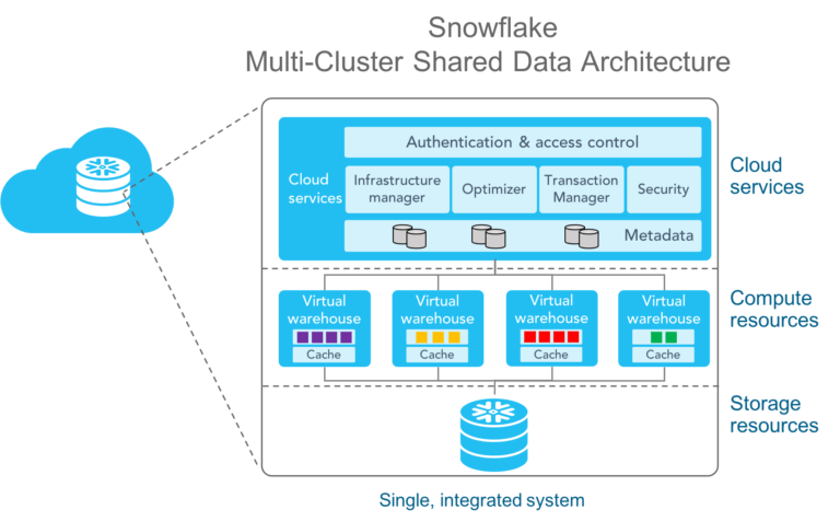
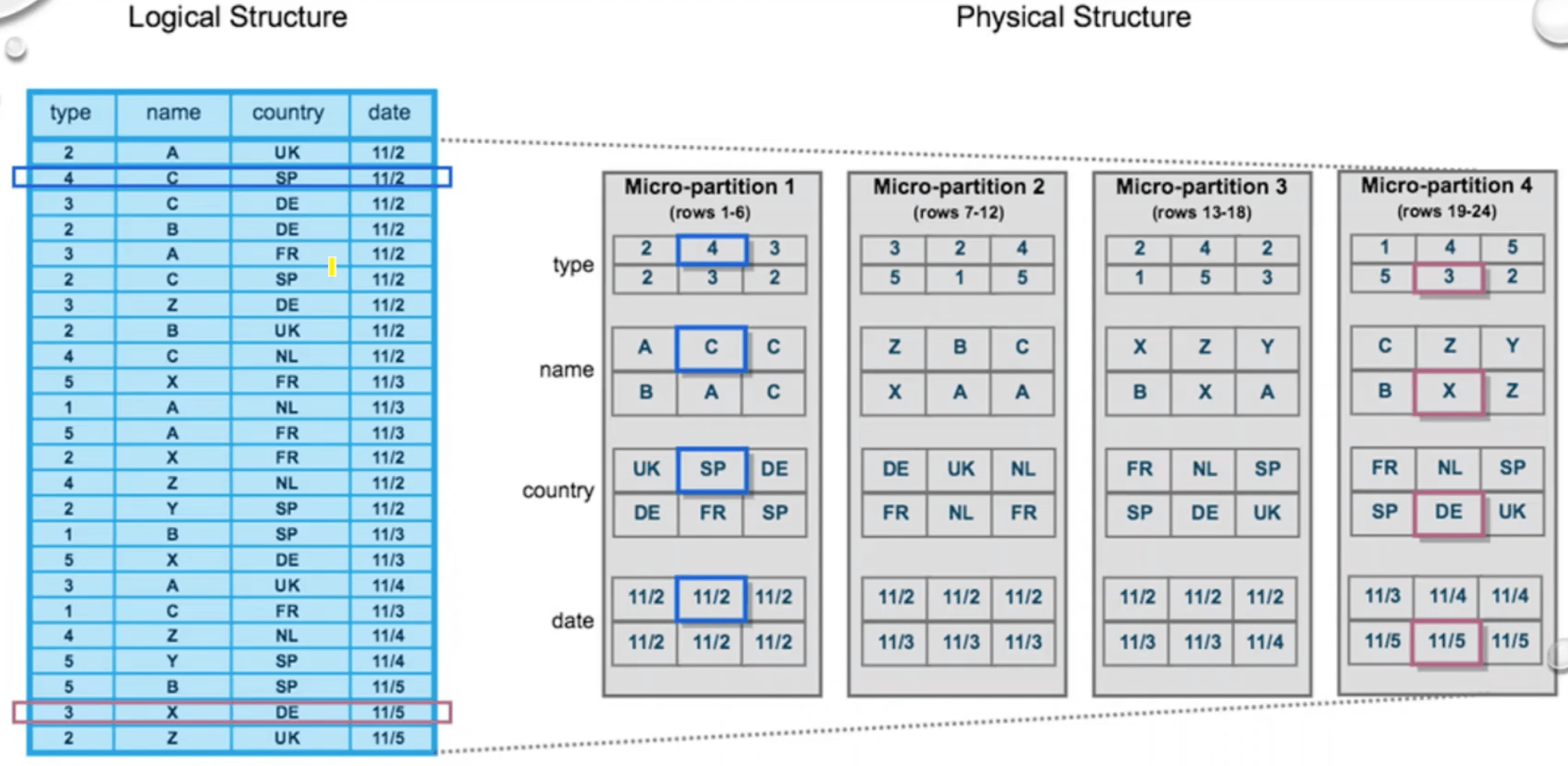
The first and outermost layer is the cloud service level, where customer requests arrive. With Node.js, Python, or lots of other connectors, customers can dial into the service level and place a query. This query is compiled and optimized using Snowflake’s metadata management, which will be explained in this article. The service level has all transactional support, as well as all security controls such as role-based access control and encryption key management. The compiled and optimized query results in a query plan. Cloud services layer(brain) stores the metadata about each micro-partition (range of valuesof each column, # of distinct values, and additional properties for optimization and efficient query processing). Each micro partition is between 50 - 500 MB in size before compression. Coulmns are independently stored with micro-partitions(referred as Column-storage) for efficient scanning.

This plan is sent to the second layer, the execution level. It takes the plan and executes each action like a recipe to generate the query result.

For the entire execution, it uses data stored in the third layer on cloud storage and reads and writes metadata snippets. Important is that all files in the cloud storage are immutable. This means that a file cannot be updated once it has been created. If a file needs to be changed, a new file must be written, which replaces the old one. Virtually unlimited cloud storage allows the non-physical deletion of such files.

Metadata Management

Metadata features in Snowflake are powered by Foundation DB. The metadata read-write patterns are that of a low-latency OLTP. Snowflake algorithms are designed for OLAP. Snowflake is built as a collection of stateless services.

• The tables are immutable micro-partitions stitched together with pointers to FDB.
• Cloning copies those pointers and assigns a new table.
• Querying data of the past time( time travel) follows pointers in FDB at an older version.

Why was FoundationsDB chosen for storing metadata for Snowflake?

FDB offers a flexible Key Value store with transaction support and is extremely reliable. FDB provides sub milli-second performance for small eads without any tuning and a resonable performance for range reads. FDB also offers automatic data rebalancing and repartitioning.

What metadata is collected and stored in FDB?

A partial list of Entities that are stored in FDB includes:

• Catalog:

  • Dictionary: databases, schemas, tables, columns, constraints, fileformats, stages, data shares
  • User management: accounts, users, roles, grants

• Service:

  • Compute management: warehouses, compute servers, storage servers
  • Storage: volumes, files, column stats

• Runtime:

  • Jobs: jobs, job queues, sessions
  • Transactions: transactions, locks

Data Manipulation Language operations

All queries that insert, update, or delete data are called Data Manipulation Language operations (DMLs). The following describes how this is done in Snowflake using metadata management.

If a table has to be created in Snowflake, for instance, by a copy-command, the data will be split into micro partitions or files, each containing a few entries. In addition, a metadata snippet is created that lists all added or deleted files as well as statistics about their contents, such as minimal-maximal-value-ranges of each column. The DML "copy into t from @s" can be used as an example of how metadata creation works. It creates a new table t from stage s. In this example, the table t contains six entries and is divided into two files - File 1 and File 2. Then the following metadata snippet is created, documenting that File 1 and File 2 have been added, and each contains uid and name in a specific range.

When inserting new entries into an existing table, it is essential to remember that files are unchangeable. This means that the new values cannot simply be added to the existing files. Instead, a new file must be created that contains the new values and expands the table in this way. Also, a new metadata snippet is added that records the added file and statistics about the data in this new file, such as minimal-maximal-value-ranges of each column.

If an entry in a table must be deleted, again, the file containing this entry cannot be changed directly. Alternatively, this file is replaced by a new one. To do this, all entries of the old file, except the one to be deleted, are copied to the new file. A new metadata snippet marks the old file as deleted, while the new one is added. Some statistics about the entries of the new file are also written to the metadata snippet.

With each new DML, a new metadata section is added, documenting which actions were performed by the DML and which new statistics apply. How this metadata management enables increased query performance will be explained in the following.

Select, Pruning, Time Travel and Cloning

Snowflake provides basic functionalities of query-based languages like select as well as special operations like time travel and zero-copy cloning. For all those operations, it uses metadata information to reduce the number of files to be queried. As a result, fewer files need to be loaded from cloud storage and scanned, which significantly improves query performance.

SELECT

If a user queries a table so that the query could look like “SELECT * FROM table t”, the query optimizer first computes a scan set. This is the reduced set of files that is actually relevant for calculating the search result. Using the t table, the scan set of the above query would include all files that are marked as added but not deleted in the metadata snippets, namely File 1, File 3, and File 4. Since the query does not contain a WHERE clause, there is nothing else to do except to send the scan set together with the query plan to the execution level to process it.

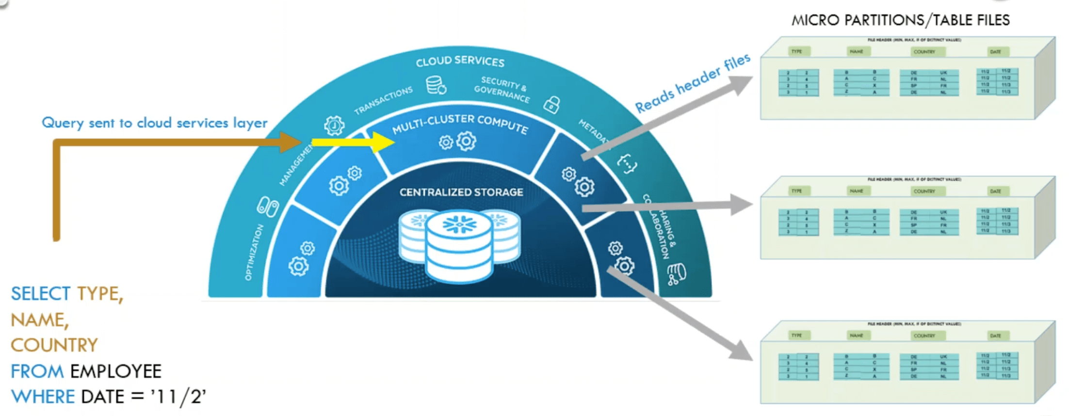
PRUNING

If a query has a pruning predicate, such as the query “SELECT * FROM table t WHERE user ID = 5”, the same scan set as described above is generated in the first step. The statistics of each file contained in the metadata snippets are then used to reduce the scan set further. These statistics include the range of values for each column of a file. With this knowledge, Snowflake can easily compare the pruning predicate, user ID = 5, with these ranges. This way, it is possible to determine the file that actually contains the desired value; here, it is File 4. Now only this single file has to be processed in the execution layer, which is much faster than scanning all files of the original scan set.

TIME TRAVEL

Another function is time travel. Since the metadata sections can also contain timestamps, users can select files that existed at a specific time. This means that if a file is deleted at 3 pm and a user then asks for all the files that existed at 2 pm, he will also receive the deleted file. This is only possible because Snowflake never physically deletes a file, but only marks it as deleted. A corresponding query could look like “SELECT * FROM table t at (timestamp =>'2pm')”. In detail, the scan set is reduced to the state of the given timestamp before either an additional pruning predicate is executed or the query is sent to the execution level. For Snowflake users, this function is limited to 24 hours by default, allowing users to revoke any modifications made in this timeframe.

ZERO COPY CLONE

The zero-copy clone is a feature that extends the SQL standard to enable table cloning in a memory-saving and performant manner. Here, no real data is cloned in the cloud, only the metadata of the files. Hence the term zero-copy. An example would be the query “Create table t2 clone table t”. To perform such an operation, all metadata snippets of the source table t are combined in a new metadata snippet. This metadata is then assigned to the new table t2 and will be the basis for all future queries on this table. In combination with the time travel function, this technique allows the user to create a zero-copy clone of a table with its contents at a specific time. This can be useful for backup or testing purposes.

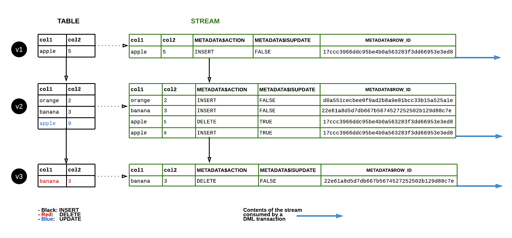
STREAMS and CDC

A stream is a new Snowflake object type that provides change data capture (CDC) capabilities to track the delta of changes in a table, including inserts and data manipulation language (DML) changes, so action can be taken using the changed data.

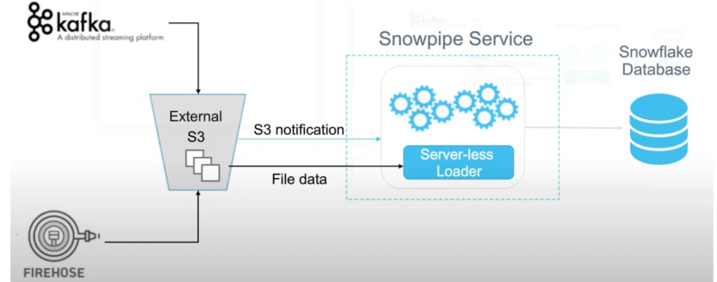
SNOWPIPE and Continuous data integration

Snowpipe is an automated service built using Amazon SQS and other Amazon Web Services (AWS) solutions that asynchronously listen for new data as it arrives to Amazon Simple Storage Service (Amazon S3) and regularly loads that data into Snowflake.

To improve the query runtime when pruning, Snowflake has implemented automatic clustering.

Automatic Clustering

While the first part of the talk explains how Snowflake stores data and manages metadata, the second part is about its automatic clustering approach. Clustering is a vital function in Snowflake because pruning performance and impact depend on the organization of data.

Naturally, the data layout (“clustering”) follows the insertion order of the executed DML operations. This order allows excellent pruning performance when filtering by attributes like date or unique identifiers if they correlate to time. But if queries filter by other attributes, by which the table is not sorted, pruning performance is unfortunate. The system would have to read every file of the affected table, leading to poor query performance.

Therefore, Snowflake re-clusters these tables. The customer is asked to provide a key or an expression that they want to use to filter their data. If this is an attribute that does not follow the insertion order, Snowflake will re-organize the table in its backend based on the given key. This process can either be triggered manually or scheduled as a background service.

The overall goal of Snowflakes clustering is not to achieve a perfect order, but to create partitions that have small value ranges. Based on the resulting order of minimal-maximal-value-ranges, the approach aims to achieve high pruning performance.

The crucial part of this algorithm is the partition selection. For this step, Snowflake is using metrics.

• One of those is the “width” of a partition. The width is of the line connecting the minimal and maximal values in the clustering values domain range. Smaller widths are beneficial since they reduce the chance that a file is relevant for a high amount of queries. That is why minimizing the partitions’ width leads to a higher pruning performance on average. The idea is to re-cluster the files that have the widest width, while this is inefficient when the data domain is very sparse.

• The second metric that Snowflake primarily uses is “depth.” This metric is the number of partitions overlapping at a specific value in the clustering key domain value range. The use of depth is based on the insight that the performance decreases when a query scans several partitions. The more files are touched, the worse is the pruning efficiency. To get consistency in that manner, Snowflake systematically reduces the worst clustering depth. All metadata is read, checking the value ranges. That way, depth peaks, in which the overlap is over a specified target level, can be identified. The partitions belonging to these peaks will be re-clustered. However, it is essential not to re-organize small files, as they are the key to fast pruning. Modifying them could decrease performance in the worst case.

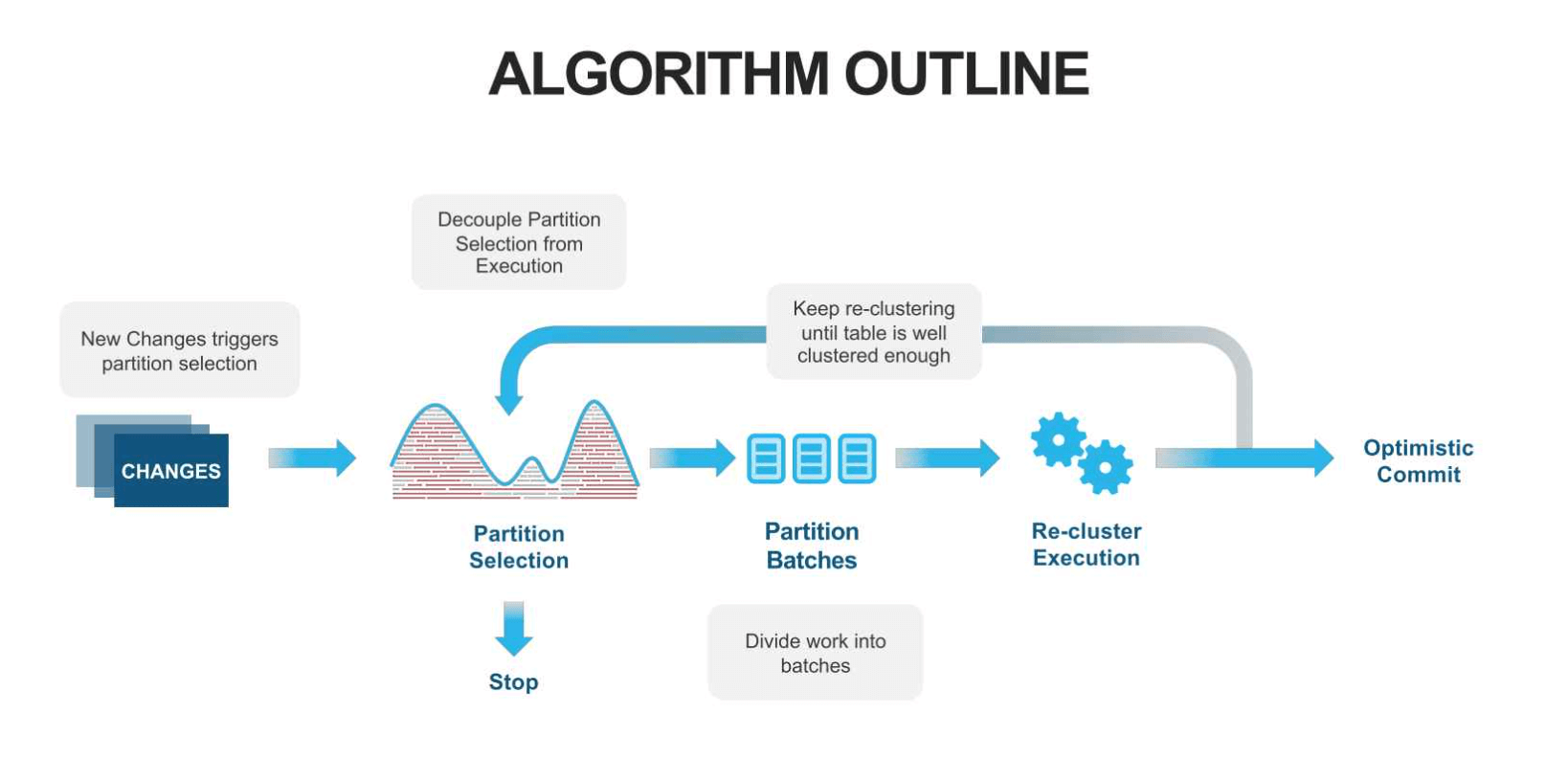
This fact is why Snowflake also takes clustering levels into account. The basic idea is to keep track of how often files have been re-clustered since this process leads to a width reduction on average. If a file has not been re-clustered yet, it is on level 0. Once re-clustered, it moves to the next level. Snowflake is using this system to ensure that files in clustering jobs have the same level. That way it provides, that already small files with excellent pruning performance do not increase their width in a cross-level re-clustering. When the customer inserts new data into Snowflake, the average query response time goes up. At the same time, the DML operations trigger background clustering jobs. Using the partition selection, Snowflake identifies the files that need to be re-clustered. After the re-clustering process, the query response time gets back down again.

Credits

🔗 Read more about Snowflake automatic clustering here

🔗 Read more about Automating Snowpipe for Amazon S3 here

Further Reading

🔗 Read more about Cassandra here

🔗 Read more about Elasticsearch here

🔗 Read more about Kafka here

🔗 Read more about Spark here

🔗 Read more about Data Lakes here

🔗 Read more about Redshift vs Snowflake here

🔗 Read more about Best Practices on Database Design here