What is Snowflake? Snowflake is an analytic data warehouse built from the ground up for the cloud to optimize loading, processing and query performance for very large volumes of data. Snowflake is a single, integrated platform delivered as-a-service. It features storage, compute, and global services layers that are physically separated but logically integrated. Data workloads scale independently from one another, making it an ideal platform for data warehousing, data lakes, data engineering, data science, modern data sharing, and developing data applications.

Auto-Clustering in Snowflake

Clustering in Snowflake is a way of organizing data in tables to make querying more efficient. It is based on the unique concept of micro-partitions, which is different from the static partitioning of tables used in traditional data warehouses. Therefore, applying clustering keys in Snowflake is also a different optimization technology compared to other database services, such as partitioning in PostgreSQL and indexing in SQL Server.

In terms of costs, data clustering in Snowflake is performed in the services layer and does not require a virtual warehouse. Snowflake keeps track of the auto-clustering service credits used in a serverless fashion. The cost of auto-clustering is a balance between credit consumption and query performance. In general, auto-clustering credit consumption is considered normal if it aligns with the DML operations on the base tables. The ultimate indicator of whether clustering is helpful or not is the query performance.

When it comes to making updates to a large amount of data, it can be beneficial to consider whether it's better to insert new records and delete old ones, or simply update the values. While inserting new records and deleting old ones will create new micro-partitions in Snowflake, so will updating values. Ultimately, the impact on clustering is similar between these methods.

However, if updates are happening very frequently (e.g. every 5 minutes), it can lead to Snowflake having to build a lot of micro-partitions, even if only a small percentage of values are being updated. In this case, it may be worthwhile to explore alternative approaches, such as relaxing the materialization schedule for the table to once per day and creating a "real-time" view that joins a snapshot table with an incremental one. This can help balance the cost of re-clustering with performance gains from the queries.

In Snowflake, there is no such thing as partial re-clustering. When you define a clustering key on a table, the automatic clustering algorithm will run on the whole column and re-cluster wherever possible based on the frequency of DMLs on the table. From a user perspective, this process is a black box. Even if only one out of ten users in a table is doing daily updates, re-clustering will occur as a normal practice to ideally cluster the table.

It is generally not a good idea to include Null values in the clustering key column, as it can cause micro-partitions to overlap and result in an poorly-clustered table.

Whether or not to cluster a table depends on various factors, such as the cardinality of the column being filtered on by DMLs, the frequency of the DMLs, and the nature of the data. It can be beneficial to separate daily, weekly, and monthly data to make a trade-off on whether to trigger clustering on updated data. However, this may not always be possible depending on the needs and design of the data pipeline.

Query Performance with Clustering

Query performance is the ultimate indicator whether it is necessary to apply a clustering key or an existing clustering key is helpful or not.

How do you know if the query performance is impacted by clustering? First, check the TableScan operator in the query profile. In general, if TableScan is in the top 3 of most expensive steps, or top 5 for a complex query, you can move on to the next step. If not, then clustering is not likely the cause for poor performance, or at least not the major cause. The top 3-5 threshold may be adjusted depending on a specific case. Second, check the percentage of micro-partitions assigned and scanned. In general, if the number of micro-partitions scanned out of the total number of micro-partitions is over 50%, we consider pruning is bad and clustering plays an important role in such cases. The 50% threshold may be adjusted depending on a specific case. Finally, reference any existing performance metrics dashboard to look for other potential issues related to clustering.

Auto-Clustering Concerns

You could have concerns about auto-clustering activities including credit consumption concern, clustering not working as expected or clustering not being able to keep up with user DMLs, etc. Auto-clustering service will try to re-cluster the table until the cost of additional micro-partition shuffling is not worth it for the defined clustering keys. This means when the table is in a stable state of clustering, only new DML operations can trigger auto-clustering, thus leading to credit consumption. If the auto-clustering activities align with user DML operations, we can generally consider the situation is working as expected. This trend between clustering and DMLs can be compared in the following aspects.

A sample query could look like this:
// Clustering activities trend select
to_date(start_time) as by_date,  sum(num_rows_reclustered) as tol_num_rows_reclustered, sum(num_bytes_reclustered) as tol_num_bytes_reclustered from snowflake.account_usage.automatic_clustering_history where true
and start_time >= dateadd(day, -14, current_date) and database_name = 'DEMO'
and schema_name = 'SAMPLE_DATA' and table_name = 'ORDERS'
group by 1
order by 1
;
// DML operations trend

select
to_date(start_time) as by_date,
sum(rows_inserted + rows_updated + rows_deleted) as tol_rows_changed, sum(bytes_written + bytes_deleted) as tol_bytes_changed
from snowflake.account_usage.query_history where true
and start_time >= dateadd(day, -14, current_date) and database_name = 'DEMO'
and schema_name = 'SAMPLE_DATA'
and query_type in ('INSERT','UPDATE','DELETE','MERGE','TRUNCATE','COPY','ALTER')
and query_text ilike '%orders%' group by 1
order by 1
;

Does the Clustering vs DMLs trend align?

 Yes

● Auto-clustering is working as expected and there is no action needed

● If you think the cost of auto-clustering is too high, revisit How To Choose Clustering Keys and determine if the defined clustering key is best balanced between query workloads and DML operations

  No

● Check if your clustering key design aligns with the best practices mentioned at How To Choose Clustering Keys

● Check the DML operations on the target table and reconsider the clustering key design

● Are there too many churns?

● Is the DML too frequent for the auto-clustering service to catch up?

● Check monitoring result mentioned at How To Monitor Clustering and Performance and see if the there is any unusual activities

● File a ticket to Snowflake Support if you still need additional help

● You think auto-clustering service is re-clustering way more than what you’ve expected

● You need additional information to determine if the trend aligns. Apart from rows and bytes changed, there are metrics such as files changed, which is not visible to Snowflake users.

Choose Clustering Key

The major factors to consider how to choose a clustering key include: Query workload Data characteristics DML operations

Query Workload

Applying clustering keys should focus on benefiting query workloads instead of tables at rest. First of all, analyze in your Snowflake environments, the important query workloads based on frequency of execution and business impact. Then you can choose clustering key columns that are most commonly used in the logical predicates and filters among these queries.

Example 1: Fact tables are commonly involved in date based queries with filters like where order_date > x and order_date <=y. The date attribute order_date can be a good candidate for clustering key columns.

Example 2: Event tables are commonly filtered by even_type = n. The event attribute event_type can be a good candidate for clustering key columns.

Any columns in the predicates can be included in a clustering key. While there is still room for additional clustering keys, you can consider columns frequently used in join predicates and aggregated columns.

Example 1: With join conditions like from table_1 join table_2 on table_1.column_a = table_2.column_b, consider column_a and column_b clustering key column candidates.

Example 2: With aggregation on a group by column_c, consider column_c a clustering key column candidate.

Data Characteristics

The most important data characteristics we care about is the number of distinct values, i.e. cardinality in a column or expression. It is important to choose a clustering key that has, A large enough number of distinct values to enable effective pruning on the table. A small enough number of distinct values to allow Snowflake to effectively group rows in the same micro-partitions.

The data distribution of the candidate columns is also important to the clustering decision. Apart from the cardinality in each column, there is the number of rows remaining after each predicate is applied that we care about.

Here are some examples to find the cardinality and selectivity of a candidate column. // cardinality select distinct <columnname> from <table_name>; // selectivity select count(distinct <column_name>)_100.0/count() from <tablename>; // data distribution select <column_name>, count() from <tablename> group by <table_name>; // number of rows on column select count() from <table_name> where <column_name> = 'xxx';

As a general rule, assuming candidate columns with moderate cardinality, make the column with the lowest number of distinct values the leading clustering key. For example, if you have a column for gender which only has 2 values, the gender column won’t be a good candidate due to its selectivity. Also, it makes more sense to choose columns in equality predicates over columns in range predicates as clustering keys since equality predicates provide more pruning.

DML Operations

DML operations have a significant impact on clustering key selection and they vary in sizes and frequencies. In general, if the DML happens on a different dimension compared to the clustering keys for the target table, maintaining the clustering on the table could be expensive.

Example 1: Assume the DML workloads are daily ETL flow based on a date column on the table, and the job adds a new date value for each day. When the table is clustered on the same date column, the data can be nicely appended to the end of the last micro-partition without impacting existing micro-partitions. Since the DML workloads are based on date, it makes sense to define the date column as the leading clustering key. As a result, daily data loads are appended to existing micro-partitions with minimal, if any, re-clustering required. Since the existing data is already mostly clustered on date and the DML is also based on date, clustering can be maintained with very little overhead. Usually, date/time columns are good candidates for leading clustering keys since the data is often loaded in order of time.

Example 2: Assume the DML workloads are daily ETL flow based on an ID column and the table is still clustered on the date column. If the ID is evenly distributed across all date values, then an ID data set introduced in the daily ETL flow could touch any number of dates. Since the table is clustered by date, re-clustering needs to touch many existing micro-partitions to maintain the ordering in the table. In this case, it might make more sense to define the ID column as the leading clustering key.

On the other hand, it is also possible to align your DML operations to the existing clustering keys on a table. There are cases you might want to consider adding an order by in your DML operation so that the data is loaded in the order of an existing clustering key on the target table. This is also a common method to prepare a table with a clustering key order without having to wait for the auto-clustering service to kick in.

create or replace table source_t (col_1 varchar, col_2 date) cluster by (col_1);
// standard way to change the clustering key for a new table
create or replace table target_t clone source_t; alter target_t cluster by col_2;

// using dml to handle the change of clustering key for a new table create or replace table target_t as select \* from source_t order by col_2; alter target_t cluster by col_2;

In some scenarios, using DML to manually populate a clustered table could be less expensive compared to keeping the re-clustering service busy for a long period of time. However, the order by can be a memory-intensive operation and not applicable to very large tables if the warehouse provisioned is not big enough.

In summary, Snowflake recommends the following strategy for determining clustering keys and maintaining the clustering for a table. Determine the queries that are most important, or most frequently executed, and then analyze predicates in these queries to determine candidate clustering keys. Look at the data characteristics of candidate columns, such as the number of distinct values. The columns with fewer distinct values should come earlier in the clustering key order. DML operations can have a big impact on the cost of maintaining a table’s clustering order. Choose clustering key columns based on a balance between query workload and DML patterns.

Summary of Considerations

It's important to keep in mind that the main reason for applying clustering keys on tables is to improve query performance. If there are no performance issues, there is no need to enforce clustering on a table. This means that you don't have to worry about the clustering depth being too high if there is no performance degradation. It is recommended to have a maximum of 3-4 columns or expressions for clustering keys on a table. Adding more than that can increase the cost without providing a significant benefit. With more clustering key columns, the overhead of maintaining the clustering order of a table tends to grow. The cost of managing the additional ordering through re-clustering may outweigh the benefits of clustering on query performance.

The order of columns does matter when defining multi-column clustering keys on a table. Snowflake generally recommends ordering the columns from lowest cardinality to highest cardinality, assuming the distribution is relatively even. In some cases, this may not apply if you consider the balance between query workload and DML patterns. However, putting a higher cardinality column before a lower one will generally reduce the effectiveness of clustering on the latter column. Numeric and date/time data types are generally more efficient than strings. When working with date/time data, consider using the date, time, or timestamp data types instead of their equivalent string values. Regular columns are generally more efficient than variant columns, as more casting is required to extract the variant elements.

Only the first 6 characters are used when the auto-clustering service operates on a table.

Rule of thumbs when you define a clustering key

Pursue clustering a table only when there is performance concern Keep the number of clustering key under 3 to 4 columns, preferable 3 at most Choose the order of clustering keys carefully Choose numeric and date time data types over string Use date/time as the leading clustering key columns if your data is loaded in order of time Use an expression such as TO_DATE() to cast timestamp to date when Timestamp data type column is in the clustering key Use an expression such as SUBSTR() to truncate commonly leading characters when a string data type column in the clustering key Pick a clustering depth for a table that achieves good query performance and re-cluster the table if it goes above the target depth

How To Understand Clustering Information

Understanding how to read the output of SYSTEM$CLUSTERING_INFORMATION is critical to the planning of a clustering strategy that optimizes performance while minimizing reclustering costs. This guidance is intended to decipher the Snowflake clustering information and practical effect of what the output means, and how to use the information to plan the clustering of Snowflake tables.

We will use a sample dataset provided by Snowflake to walk through a user’s journey of understanding clustering information. Note that using the TPCH sample data in this guidance (approx. 50GBs) will incur credit consumption. It is not necessary to run the scripts unless you would like to experiment and see it on your own.

create or replace database demo;
create or replace schema demo.sample_data;
create or replace table demo.sample_data.orders_sorted as select \* from sample_data.tpch_sf1000.orders
order by o_orderkey
;

The above scripts create an orders_sorted table that has a natural clustering arrangement on the o_orderkey column in its perfectly sorted state.

Return Clustering Information

To return clustering information, use the system function following the syntax shown in Snowflake documentation. Note that the column augment can be used to return clustering information for any column in the table, regardless if a clustering key is defined for the table, or if the column is part of the clustering key. We can test a “what-if“ key against an existing table with data that helps you decide the clustering key.

select system$clustering_information('orders_sorted','(o_orderkey)');

Using the command above against our sample dataset produces the following clustering information output.

{
  "cluster_by_keys": "LINEAR(o_orderkey)",
  "notes": "Clustering key columns contain high cardinality key O_ORDERKEY which might result in expensive re-clustering. Consider reducing the cardinality of clustering keys. Please refer to https://docs.snowflake.net/manuals/user-guide/tables-clustering-keys.html for more information.",
  "total_partition_count": 2488,
  "total_constant_partition_count": 0,
  "average_overlaps": 0.0,
  "average_depth": 1.0,
  "partition_depth_histogram": {
    "00000": 0,
    "00001": 2488,
    "00002": 0,
    "00003": 0,
    "00004": 0,
    "00005": 0,
    "00006": 0,
    "00007": 0,
    "00008": 0,
    "00009": 0,
    "00010": 0,
    "00011": 0,
    "00012": 0,
    "00013": 0,
    "00014": 0,
    "00015": 0,
    "00016": 0
  }
}

It is important to know that the output is not guaranteed to show up-to-date information. If you test on a “what-if“ key, it may default to showing the worst case clustering until the table is re-clustered using the key at least once. In general, if testing a “what-if“ key, the result is

Read the Output Snowflake documentation has a high level description of the output. To decipher the output in detail, we need to understand the nature of the output from the system function. The function is a metadata only operation The statistics indicate how well a table is clustered based on a specific clustering key The statistics indicate the current clustering state on a key, or what the state might be if clustered on a different key

When we created the table, it was sorted on o_orderkey. Thus, even though we haven’t explicitly defined a clustering key, the output of SYSTEM$CLUSTERING_INFORMATION shows a best case scenario of clustering arrangement on a “what-if“ o_orderkey clustering key. The function analyzes the clustering arrangement for the o_orderkey attribute by taking each micro-partition’s min and max values and traversing the other micro-partitions to find where its min and max intersect with the other micro-partitions. This intersection is referred to as an overlap as the range of one micro-partition’s min and max values overlap with another’s range.

All micro-partitions overlap (average_overlaps = total_partition_count - 1

Average depth is exactly the number of total micro-partitions

Histogram shows all micro-partitions in the bin that is the next power of 2 higher than the partition count

This comparison output shows how efficiently Snowflake optimizer can prune partitions when using the tested clustering key as a filter. We can use a simple statement as an example to compare the query result.

select * from orders_sorted where o_orderkey = 1324096740;

Selecting with a filter on o_orderkey in the best case scenario, the query took about 1 second on an XS warehouse and scanned exactly 1 micro-partition.

The optimizer was able to exclude all other micro-partitions from scanning because there are no overlaps in the table with such clustering arrangement over o_orderkey.

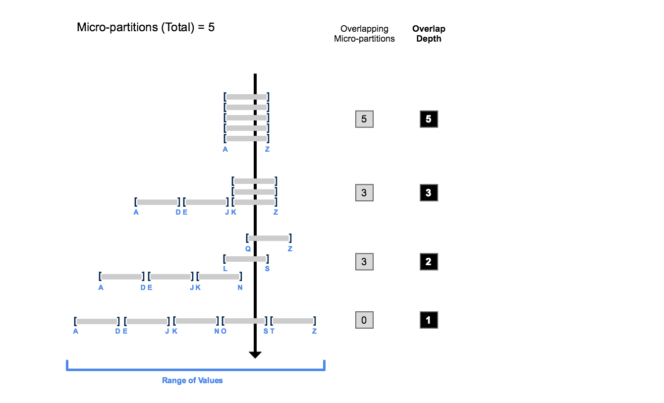
Zoom in the clustering depth using the Snowflake “stab analysis“ infographic, you can see what average_depth means and what’s happening when a query filtered on o_orderkey runs against the table.

To illustrate the other extreme, consider a table that has clustering on the same o_orderkey but as bad as it can be. We can create another table and this time order by a random number over o_orderkey

create or replace table demo.sample_data.orders_randomized as select * from sample_data.tpch_sf1000.orders order by random();

If we run the SYSTEM$CLUSTERING_INFORMATION function again, we are looking at completely different output.

select system$clustering_information('orders_randomized','(o_orderkey)');

Comparing a best case scenario of clustering arrangement on o_orderkey side-by-side with a worst-case scenario on the same attribute.

No overlapping micro-partitions Average depth is exactly 1.0 Histogram shows that all micro-partitions in the “00001” bin

{
  "cluster_by_keys": "LINEAR(o_orderkey)",
  "notes": "Clustering key columns contain high cardinality key O_ORDERKEY which might result in expensive re-clustering. Consider reducing the cardinality of clustering keys. Please refer to https://docs.snowflake.net/manuals/user-guide/tables-clustering-keys.html for more information.",
  "total_partition_count": 2680,
  "total_constant_partition_count": 0,
  "average_overlaps": 2679.0,
  "average_depth": 2680.0,
  "partition_depth_histogram": {
    "00000": 0,
    "00001": 0,
    "00002": 0,
    "00003": 0,
    "00004": 0,
    "00005": 0,
    "00006": 0,
    "00007": 0,
    "00008": 0,
    "00009": 0,
    "00010": 0,
    "00011": 0,
    "00012": 0,
    "00013": 0,
    "00014": 0,
    "00015": 0,
    "00016": 0,
    "04096": 2680
  }
}

All micro-partitions overlap (average_overlaps = total_partition_count - 1) Average depth is exactly the number of total micro-partitions Histogram shows all micro-partitions in the bin that is the next power of 2 higher than the partition count

This comparison output shows how efficiently Snowflake optimizer can prune partitions when using the tested clustering key as a filter. We can use a simple statement as an example to compare the query result.

select \* from orders_sorted where o_orderkey = 1324096740;

Selecting with a filter on o_orderkey in the best case scenario, the query took about 1 second on an XS warehouse and scanned exactly 1 micro-partition.

The optimizer was able to exclude all other micro-partitions from scanning because there are no overlaps in the table with such clustering arrangement over o_orderkey

select * from orders_randomized where o_orderkey = 1324096740;

Running the same query with the same warehouse in the worst case scenario, the query took 18 seconds and scanned all 2680 micro-partitions.

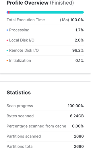
The optimizer had to scan all of the micro-partitions because the o_orderkey value in the where predicate exists within each of their min and max range.

Metrics

| Stats | Description | | ------------------------------ | --------------------------------------------------------------------------------------------------------------------------------------------------------------------------------------------------------------------------------------------------------------------------------------------------------------------------------------------------------------------------------------------------------------------------------------------------------------------------------------------------------------------------------------------------------------------------- | | cluster_by_keys | This is the key tested when the function is running, not necessarily the current keys used for clustering | | LINEAR | This is the re-clustering method. Since it is currently the only method, it will always display as LINEAR | | o_orderkey | This is the expression tested, not necessarily the currently defined clustering key | | note | There is a note about expensive re-clustering because o_orderkey is a high cardinality attribute. In a real world scenario, it is best to re-evaluate the key selection following the clustering key selection strategy. We are going to ignore it since the example is an extreme case to help illustrate clustering states | | total_partition_count | This shows the current total partition count, not including partitions needed for time travel and fail safe | | total_constant_partition_count | The is the number of micro-partitions that are effectively in an optimal state and will not benefit from additional re-clustering operations | | average_overlaps | This indicates how many other partitions on average a partition's min and max values overlap. Since the table was created by sorting on o_orderkey and the attribute is an unique column, the min and max values of the micro-partition don’t overlap at all. | | average_depth | This shows the average of overlap depth for each micro-partition, which is best illustrated in the stab analysis from Snowflake doc | | partition_depth_histogram | This is an example of a well clustered table based on o_orderkey. The first bin, “00000” will always be 0 as by definition, a cluster depth must be a minimum of 1. The histogram always displays bins 1 through 16, and will display in powers of two until accounting for all micro-partitions. It will not, however, display any bins beyond “00016” that have zero values. After displaying bin “00016”, if necessary, the function displays bins in powers of 2, 32, 64, 128, and so on. If a bin greater than “00016” is zero, the histogram omits this bin entirely. |

Metadata Management

This plan is sent to the second layer, the execution level. It takes the plan and executes each action like a recipe to generate the query result.

For the entire execution, it uses data stored in the third layer on cloud storage and reads and writes metadata snippets. Important is that all files in the cloud storage are immutable. This means that a file cannot be updated once it has been created. If a file needs to be changed, a new file must be written, which replaces the old one. Virtually unlimited cloud storage allows the non-physical deletion of such files.

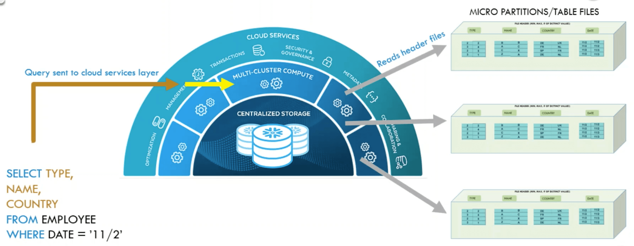
Metadata features in Snowflake are powered by Foundation DB. The metadata read-write patterns are that of a low-latency OLTP. Snowflake algorithms are designed for OLAP. Snowflake is built as a collection of stateless services.

• The tables are immutable micro-partitions stitched together with pointers to FDB.
• Cloning copies those pointers and assigns a new table.
• Querying data of the past time( time travel) follows pointers in FDB at an older version.

Why was FoundationsDB chosen for storing metadata for Snowflake?

FDB offers a flexible Key Value store with transaction support and is extremely reliable. FDB provides sub milli-second performance for small eads without any tuning and a resonable performance for range reads. FDB also offers automatic data rebalancing and repartitioning.

Data Manipulation Language operations

All queries that insert, update, or delete data are called Data Manipulation Language operations (DMLs). The following describes how this is done in Snowflake using metadata management.

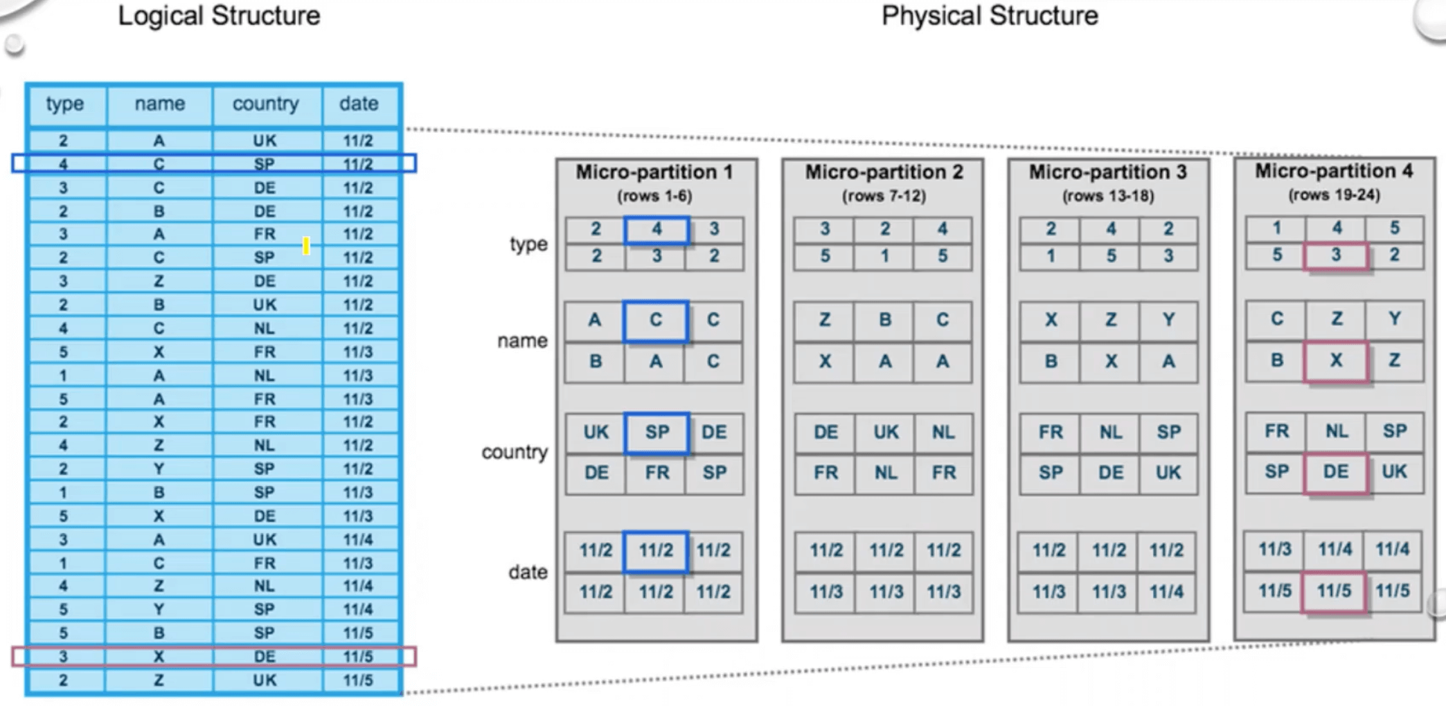
If a table has to be created in Snowflake, for instance, by a copy-command, the data will be split into micro partitions or files, each containing a few entries. In addition, a metadata snippet is created that lists all added or deleted files as well as statistics about their contents, such as minimal-maximal-value-ranges of each column. The DML "copy into t from @s" can be used as an example of how metadata creation works. It creates a new table t from stage s. In this example, the table t contains six entries and is divided into two files - File 1 and File 2. Then the following metadata snippet is created, documenting that File 1 and File 2 have been added, and each contains uid and name in a specific range.

When inserting new entries into an existing table, it is essential to remember that files are unchangeable. This means that the new values cannot simply be added to the existing files. Instead, a new file must be created that contains the new values and expands the table in this way. Also, a new metadata snippet is added that records the added file and statistics about the data in this new file, such as minimal-maximal-value-ranges of each column.

If an entry in a table must be deleted, again, the file containing this entry cannot be changed directly. Alternatively, this file is replaced by a new one. To do this, all entries of the old file, except the one to be deleted, are copied to the new file. A new metadata snippet marks the old file as deleted, while the new one is added. Some statistics about the entries of the new file are also written to the metadata snippet.

With each new DML, a new metadata section is added, documenting which actions were performed by the DML and which new statistics apply. How this metadata management enables increased query performance will be explained in the following.

Conclusion

While the first part of the talk explains how Snowflake stores data and manages metadata, the second part is about its automatic clustering approach. Clustering is a vital function in Snowflake because pruning performance and impact depend on the organization of data.

Naturally, the data layout (“clustering”) follows the insertion order of the executed DML operations. This order allows excellent pruning performance when filtering by attributes like date or unique identifiers if they correlate to time. But if queries filter by other attributes, by which the table is not sorted, pruning performance is unfortunate. The system would have to read every file of the affected table, leading to poor query performance.

Therefore, Snowflake re-clusters these tables. The customer is asked to provide a key or an expression that they want to use to filter their data. If this is an attribute that does not follow the insertion order, Snowflake will re-organize the table in its backend based on the given key. This process can either be triggered manually or scheduled as a background service.

The overall goal of Snowflakes clustering is not to achieve a perfect order, but to create partitions that have small value ranges. Based on the resulting order of minimal-maximal-value-ranges, the approach aims to achieve high pruning performance.

The crucial part of this algorithm is the partition selection. For this step, Snowflake is using metrics.

• One of those is the “width” of a partition. The width is of the line connecting the minimal and maximal values in the clustering values domain range. Smaller widths are beneficial since they reduce the chance that a file is relevant for a high amount of queries. That is why minimizing the partitions’ width leads to a higher pruning performance on average. The idea is to re-cluster the files that have the widest width, while this is inefficient when the data domain is very sparse.

• The second metric that Snowflake primarily uses is “depth.” This metric is the number of partitions overlapping at a specific value in the clustering key domain value range. The use of depth is based on the insight that the performance decreases when a query scans several partitions. The more files are touched, the worse is the pruning efficiency. To get consistency in that manner, Snowflake systematically reduces the worst clustering depth. All metadata is read, checking the value ranges. That way, depth peaks, in which the overlap is over a specified target level, can be identified. The partitions belonging to these peaks will be re-clustered. However, it is essential not to re-organize small files, as they are the key to fast pruning. Modifying them could decrease performance in the worst case.

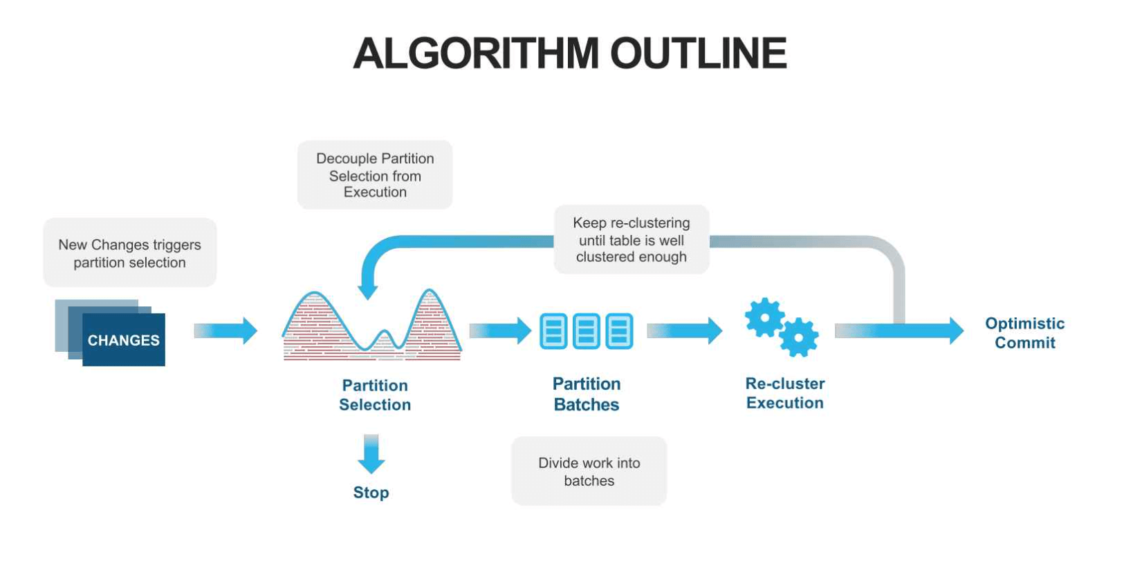
This fact is why Snowflake also takes clustering levels into account. The basic idea is to keep track of how often files have been re-clustered since this process leads to a width reduction on average. If a file has not been re-clustered yet, it is on level 0. Once re-clustered, it moves to the next level. Snowflake is using this system to ensure that files in clustering jobs have the same level. That way it provides, that already small files with excellent pruning performance do not increase their width in a cross-level re-clustering. When the customer inserts new data into Snowflake, the average query response time goes up. At the same time, the DML operations trigger background clustering jobs. Using the partition selection, Snowflake identifies the files that need to be re-clustered. After the re-clustering process, the query response time gets back down again.

Credits

🔗 Read more about Snowflake automatic clustering here